4 Background
Blastic plasmacytoid dendritic cell neoplasm (BPDCN) is an ultra-rare (≈0.05 per 100,000), aggressive hematologic malignancy involving skin, bone marrow, blood, lymph nodes, and CNS.
It is characterized by universal overexpression of CD123 (interleukin-3 receptor-α) on neoplastic blasts, making CD123 an attractive therapeutic target.
The median age at diagnosis is approximately 65–70 years, with a 3:1 male predominance.
Historically, treatment relied on chemotherapy regimens adapted from acute leukemias, yielding complete remission rates of only 41–55% with short durations and median overall survival of just 8–14 months.
Tagraxofusp became the first FDA-approved therapy for BPDCN (December 2018) and the first CD123-targeted agent approved for any indication. The EMA followed with approval in 2021 for first-line treatment in adults.
4.1 Mechanism of Action
Show code
library(ggplot2)

mechanism_data <- data.frame(
  step = factor(c(
    "1. CD123\nBinding",
    "2. Receptor\nEndocytosis",
    "3. DT Domain\nCleavage",
    "4. EF2\nInactivation",
    "5. Protein Syn.\nInhibition",
    "6. Cell\nDeath"
  ), levels = c(
    "1. CD123\nBinding",
    "2. Receptor\nEndocytosis",
    "3. DT Domain\nCleavage",
    "4. EF2\nInactivation",
    "5. Protein Syn.\nInhibition",
    "6. Cell\nDeath"
  )),
  component = c("Ligand", "Ligand", "Toxin", "Toxin", "Effect", "Effect"),
  y = c(1, 1, 1, 1, 1, 1),
  description = c(
    "IL-3 fused to\ntruncated DT",
    "Receptor-mediated\nentry into cell",
    "Catalytic domain\ntranslocates to cytosol",
    "ADP-ribosylation\nof diphthamide",
    "Disruption of\nprotein synthesis",
    "Apoptotic\ncell death"
  )
)

color_palette <- c(
  "Ligand" = "#2166ac",
  "Toxin"  = "#d6604d",
  "Effect" = "#3a3a3a"
)

ggplot(mechanism_data, aes(x = step, y = y)) +
  geom_segment(
    data = data.frame(x = 1:5, xend = 2:6, y = 1, yend = 1),
    aes(x = x, xend = xend, y = y, yend = yend),
    inherit.aes = FALSE,
    arrow = arrow(length = unit(0.25, "cm"), type = "closed"),
    color = "#888888", linewidth = 1.2
  ) +
  geom_point(aes(color = component), size = 18) +
  geom_text(aes(label = gsub("\\d+\\. ", "", gsub("\n", " ", as.character(step)))),
            size = 3, fontface = "bold", color = "white") +
  geom_text(aes(label = description, y = y - 0.15),
            size = 2.8, color = "#444444") +
  scale_color_manual(values = color_palette, name = "Component") +
  scale_x_discrete() +
  scale_y_continuous(limits = c(0.7, 1.2)) +
  labs(
    title = "Tagraxofusp (SL-401): Mechanism of Action",
    subtitle = "CD123-directed cytotoxin — IL-3/diphtheria toxin fusion protein"
  ) +
  theme_void(base_size = 13) +
  theme(
    plot.title = element_text(hjust = 0.5, face = "bold", size = 16, color = "#1a5276"),
    plot.subtitle = element_text(hjust = 0.5, size = 11, color = "#555555",
                                 margin = margin(b = 15)),
    legend.position = "bottom",
    plot.margin = margin(20, 20, 20, 20)
  )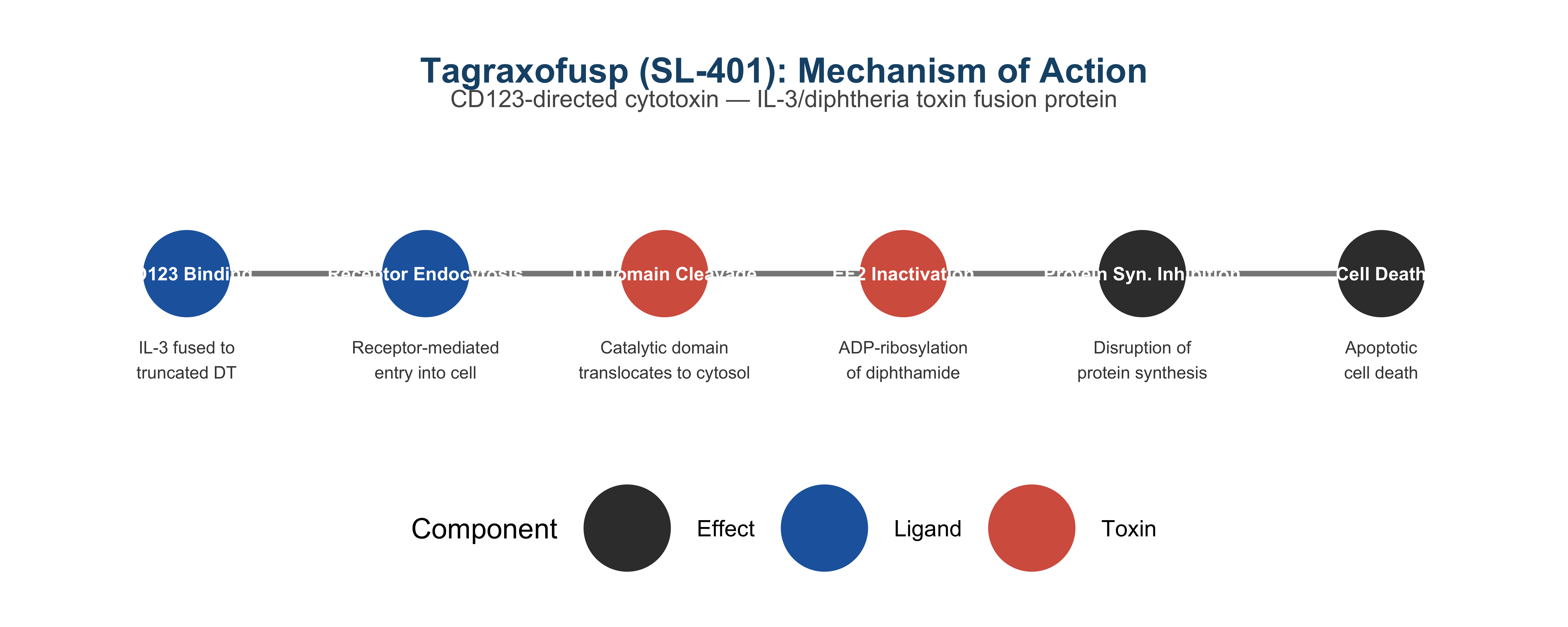
Acquired resistance to tagraxofusp does not involve loss of CD123 expression. Instead, resistance is mediated by DNA methylation–driven silencing of genes in the diphthamide synthesis pathway, rendering the diphtheria toxin payload ineffective. This mechanistic insight supports the rationale for second-line CD123-directed therapies with alternate payloads (e.g., pivekimab sunirine).
5 Study Design
The STML-401-0114 trial (NCT02113982) was a multi-stage, multi-center, open-label, phase I/II study. Patients received tagraxofusp 12 μg/kg/day IV on days 1–5 of each 21-day cycle until progression or transplant.
| Population | Description | N |
|---|---|---|
| Stage 1 | Dose-escalation (7 & 12 μg/kg) | 9 |
| Stage 2 | Expansion phase | 23 |
| Stage 3 | Pivotal phase (treatment-naïve) | 13 |
| Stage 4 | Continued-access phase | 44 |
| All Treatment-Naïve | Stages 1–4, 12 μg/kg | 65 |
| Relapsed/Refractory | All stages | 19 |
| Total (12 μg/kg) | Efficacy + safety population | 84 |
| Endpoint | Type | Definition |
|---|---|---|
| CR + CRc rate | Primary | Complete response + clinical CR (1L, stages 1–3) |
| Duration of CR+CRc | Secondary | Time from first response to relapse/death |
| OS | Secondary | Time from first dose to death |
| ORR | Secondary | CR + CRc + PR |
| Bridge to SCT | Exploratory | Patients proceeding to stem-cell transplant |
| Parameter | Specification |
|---|---|
| Dose | 12 μg/kg/day |
| Schedule | Days 1–5 of each 21-day cycle |
| Route | Intravenous infusion (15 minutes) |
| Cycle 1 setting | Inpatient (CLS monitoring) |
| Cycle 2+ setting | Outpatient permitted |
| Pre-medication | Corticosteroids, H1/H2-blockers, acetaminophen |
| Daily monitoring | Vital signs, weight, albumin, creatinine, LFTs |
| Albumin threshold | Baseline ≥3.2 g/dL required |
| Approved age | Adults + children ≥2 yr (US FDA); adults only (EMA) |
6 Patient Demographics
Show code
library(ggplot2)
library(dplyr)
library(tidyr)

demo_data <- tibble(
  Characteristic = c(
    "Age ≥65 years", "Male", "White",
    "ECOG PS 0", "ECOG PS 1",
    "Skin involvement", "Bone marrow involvement",
    "Peripheral blood", "Lymph nodes", "Visceral"
  ),
  `Treatment-Naïve\n(n = 65)` = c(62, 80, 88, 48, 48, 92, 49, 26, 51, 14),
  `Relapsed/Refractory\n(n = 19)` = c(74, 84, 90, 37, 63, 79, 63, 5, 47, 21)
)

demo_long <- demo_data |>
  pivot_longer(-Characteristic, names_to = "Group", values_to = "Percentage") |>
  mutate(
    Characteristic = factor(Characteristic, levels = rev(demo_data$Characteristic)),
    Group = factor(Group, levels = c(
      "Treatment-Naïve\n(n = 65)",
      "Relapsed/Refractory\n(n = 19)"
    ))
  )

group_colors <- c(
  "Treatment-Naïve\n(n = 65)" = "#2166ac",
  "Relapsed/Refractory\n(n = 19)" = "#d6604d"
)

ggplot(demo_long, aes(x = Percentage, y = Characteristic, fill = Group)) +
  geom_col(position = position_dodge(width = 0.75), width = 0.7, alpha = 0.9) +
  geom_text(
    aes(label = paste0(Percentage, "%")),
    position = position_dodge(width = 0.75),
    hjust = -0.15, size = 3.2, fontface = "bold"
  ) +
  scale_fill_manual(values = group_colors) +
  scale_x_continuous(
    limits = c(0, 110),
    breaks = seq(0, 100, 25),
    labels = function(x) paste0(x, "%")
  ) +
  labs(
    title = "Baseline Patient Characteristics",
    subtitle = "STML-401-0114 — Tagraxofusp in BPDCN (N = 84 at 12 μg/kg)",
    x = "Patients (%)",
    y = NULL,
    fill = "Treatment Group"
  ) +
  theme_minimal(base_size = 13) +
  theme(
    plot.title = element_text(face = "bold", size = 16, color = "#1a5276"),
    plot.subtitle = element_text(size = 12, color = "#555555", margin = margin(b = 15)),
    legend.position = "bottom",
    legend.title = element_text(face = "bold"),
    panel.grid.major.y = element_blank(),
    panel.grid.minor = element_blank(),
    axis.text.y = element_text(size = 11),
    plot.margin = margin(15, 25, 15, 15)
  )
6.1 Prior Therapies in Relapsed/Refractory Patients
Show code
import matplotlib.pyplot as plt
import numpy as np

therapies = ['1 prior line', '2–3 prior lines', '≥4 prior lines']
percentages = [58, 27, 16]

fig, ax = plt.subplots(figsize=(10, 5))

colors = ['#2166ac', '#4393c3', '#d6604d']

bars = ax.barh(
    range(len(therapies)), percentages,
    color=colors, edgecolor='white', linewidth=1.5, height=0.55
)

for bar, pct in zip(bars, percentages):
    ax.text(
        bar.get_width() + 1.5, bar.get_y() + bar.get_height()/2,
        f'{pct}%', va='center', ha='left', fontsize=12, fontweight='bold',
        color='#333333'
    )

ax.set_yticks(range(len(therapies)))
ax.set_yticklabels(therapies, fontsize=12)
ax.set_xlim(0, 75)
(0.0, 75.0)Show code
ax.set_xlabel('Patients (%)', fontsize=12)
ax.set_title(
    'Prior Lines of Therapy — Relapsed/Refractory BPDCN (n = 19)',
    fontsize=15, fontweight='bold', color='#1a5276', pad=15
)
ax.invert_yaxis()
ax.spines['top'].set_visible(False)
ax.spines['right'].set_visible(False)
ax.spines['left'].set_visible(False)
ax.tick_params(left=False)
ax.grid(axis='x', alpha=0.3, linestyle='--')

plt.tight_layout()
plt.show()
7 Efficacy Results
7.1 Response Rates
Show code
library(ggplot2)
library(dplyr)
library(tidyr)

response_df <- tibble(
  Group = factor(c(
    "Stages 1–3\n(n = 29)",
    "Overall 1L\n(n = 65)",
    "Relapsed/Refractory\n(n = 19)"
  ), levels = c(
    "Stages 1–3\n(n = 29)",
    "Overall 1L\n(n = 65)",
    "Relapsed/Refractory\n(n = 19)"
  )),
  CR_CRc = c(72, 57, 16),
  PR     = c(18, 18, 42),
  No_Response = c(10, 25, 42),
  CR_lower = c(53, 44, 3),
  CR_upper = c(87, 69, 40)
)

resp_long <- response_df |>
  select(Group, CR_CRc, PR, No_Response) |>
  pivot_longer(-Group, names_to = "Response", values_to = "Percentage") |>
  mutate(Response = factor(Response,
    levels = c("No_Response", "PR", "CR_CRc"),
    labels = c("No Response", "PR", "CR + CRc")
  ))

resp_colors <- c(
  "CR + CRc"    = "#2166ac",
  "PR"          = "#67a9cf",
  "No Response" = "#e0e0e0"
)

orr_labels <- tibble(
  Group = response_df$Group,
  ORR = c(90, 75, 58),
  y_pos = c(92, 77, 60)
)

ggplot(resp_long, aes(x = Group, y = Percentage, fill = Response)) +
  geom_col(width = 0.65, color = "white", linewidth = 0.5) +
  geom_errorbar(
    data = response_df,
    aes(x = Group, ymin = CR_lower, ymax = CR_upper, y = NULL, fill = NULL),
    inherit.aes = FALSE,
    width = 0.15, linewidth = 0.8, color = "#333333"
  ) +
  geom_text(
    data = response_df,
    aes(x = Group, y = CR_CRc / 2, label = paste0(CR_CRc, "%"), fill = NULL),
    inherit.aes = FALSE,
    color = "white", fontface = "bold", size = 6
  ) +
  geom_text(
    data = orr_labels,
    aes(x = Group, y = y_pos + 5, label = paste0("ORR: ", ORR, "%"), fill = NULL),
    inherit.aes = FALSE,
    color = "#1a5276", fontface = "bold", size = 4.2
  ) +
  scale_fill_manual(values = resp_colors, name = "Response Category") +
  scale_y_continuous(
    limits = c(0, 108),
    breaks = seq(0, 100, 25),
    labels = function(x) paste0(x, "%")
  ) +
  labs(
    title = "Best Overall Response Rates — Tagraxofusp 12 μg/kg in BPDCN",
    subtitle = "Primary endpoint: CR + CRc in previously untreated patients | Error bars: 95% CIs",
    x = NULL,
    y = "Patients (%)"
  ) +
  theme_minimal(base_size = 14) +
  theme(
    plot.title = element_text(face = "bold", size = 17, color = "#1a5276"),
    plot.subtitle = element_text(size = 12, color = "#555555", margin = margin(b = 15)),
    legend.position = "bottom",
    legend.title = element_text(face = "bold"),
    panel.grid.major.x = element_blank(),
    panel.grid.minor = element_blank(),
    axis.text.x = element_text(size = 12, face = "bold"),
    plot.margin = margin(15, 20, 15, 15)
  ) +
  guides(fill = guide_legend(reverse = TRUE))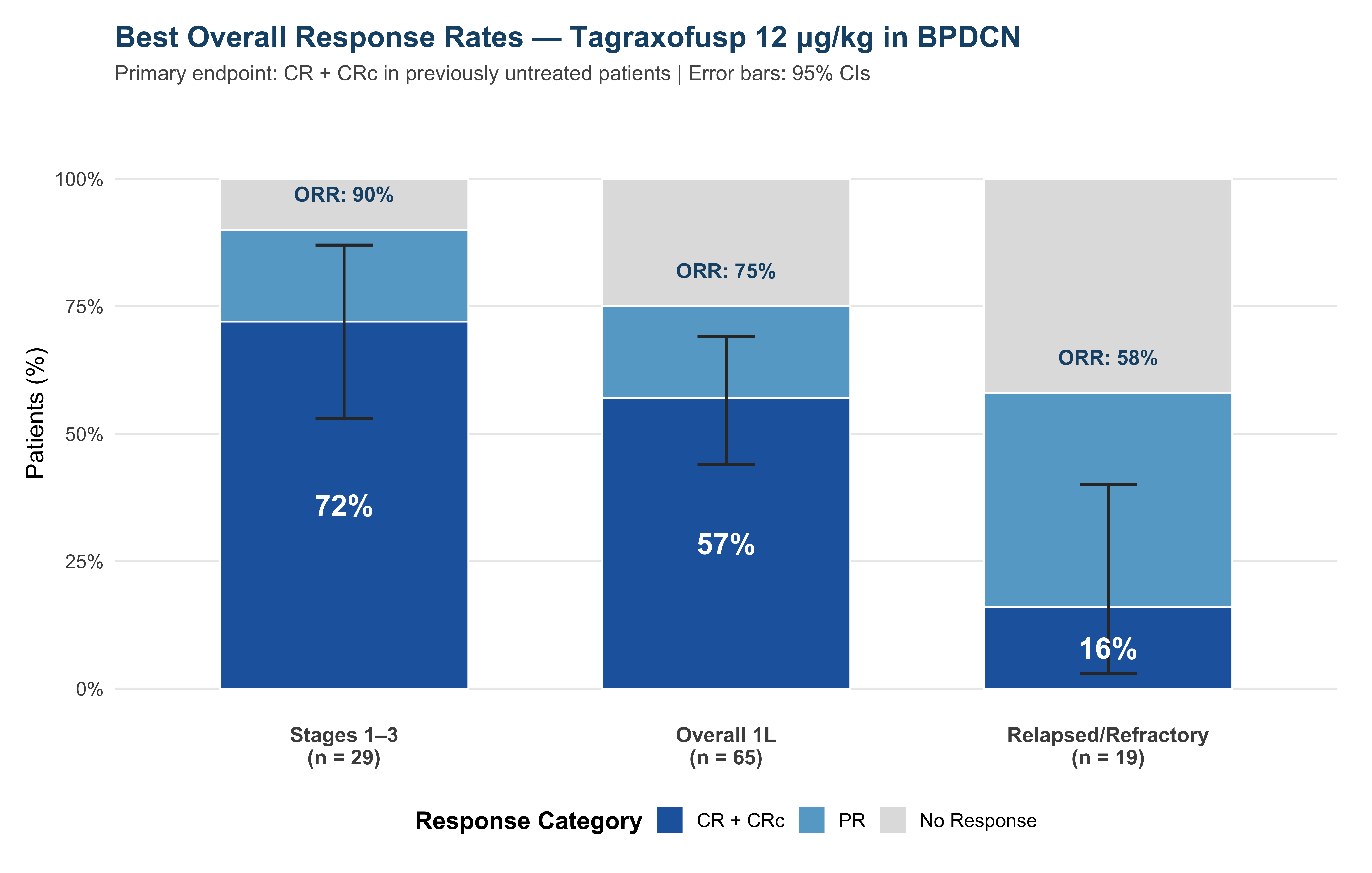
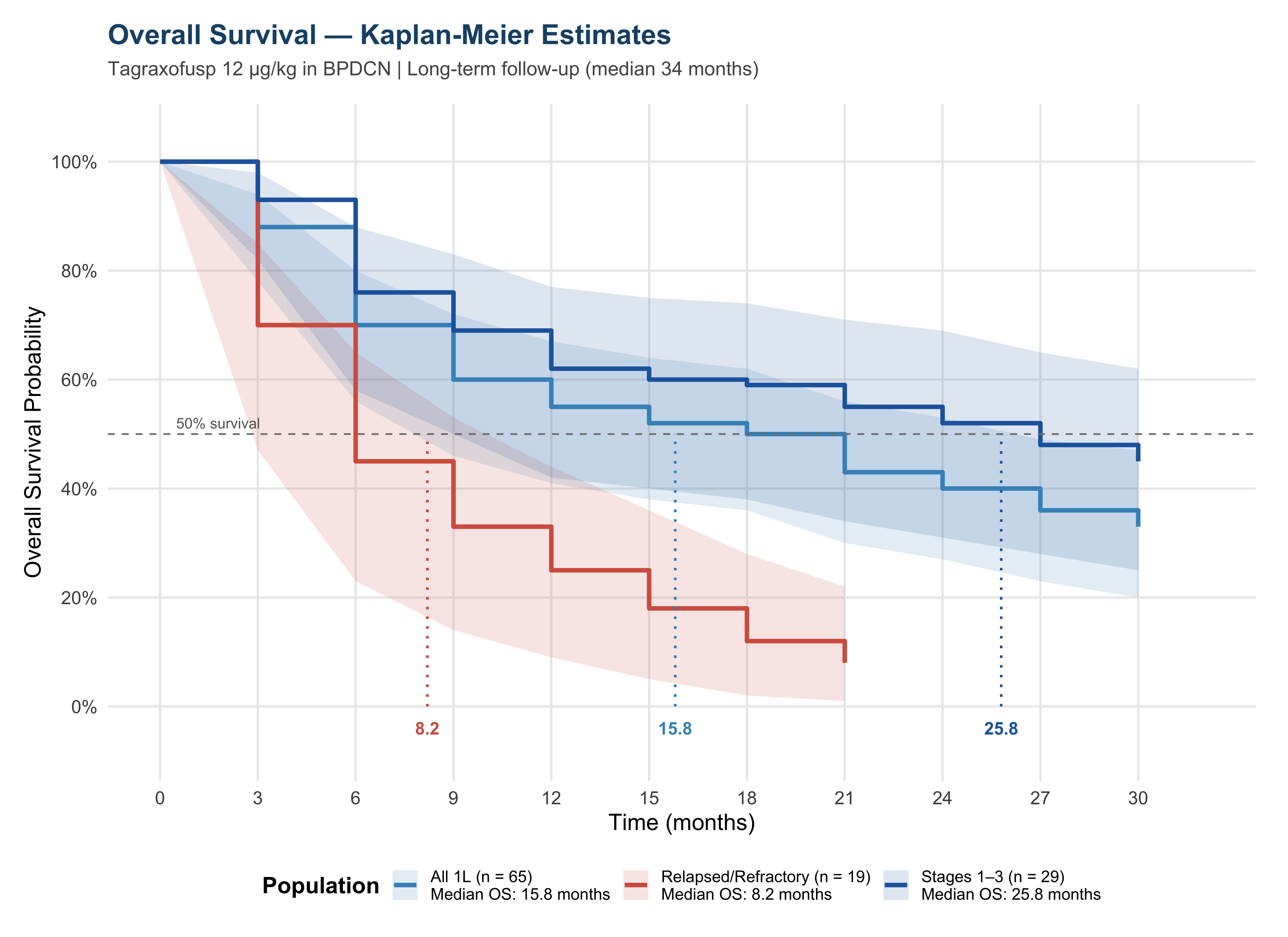
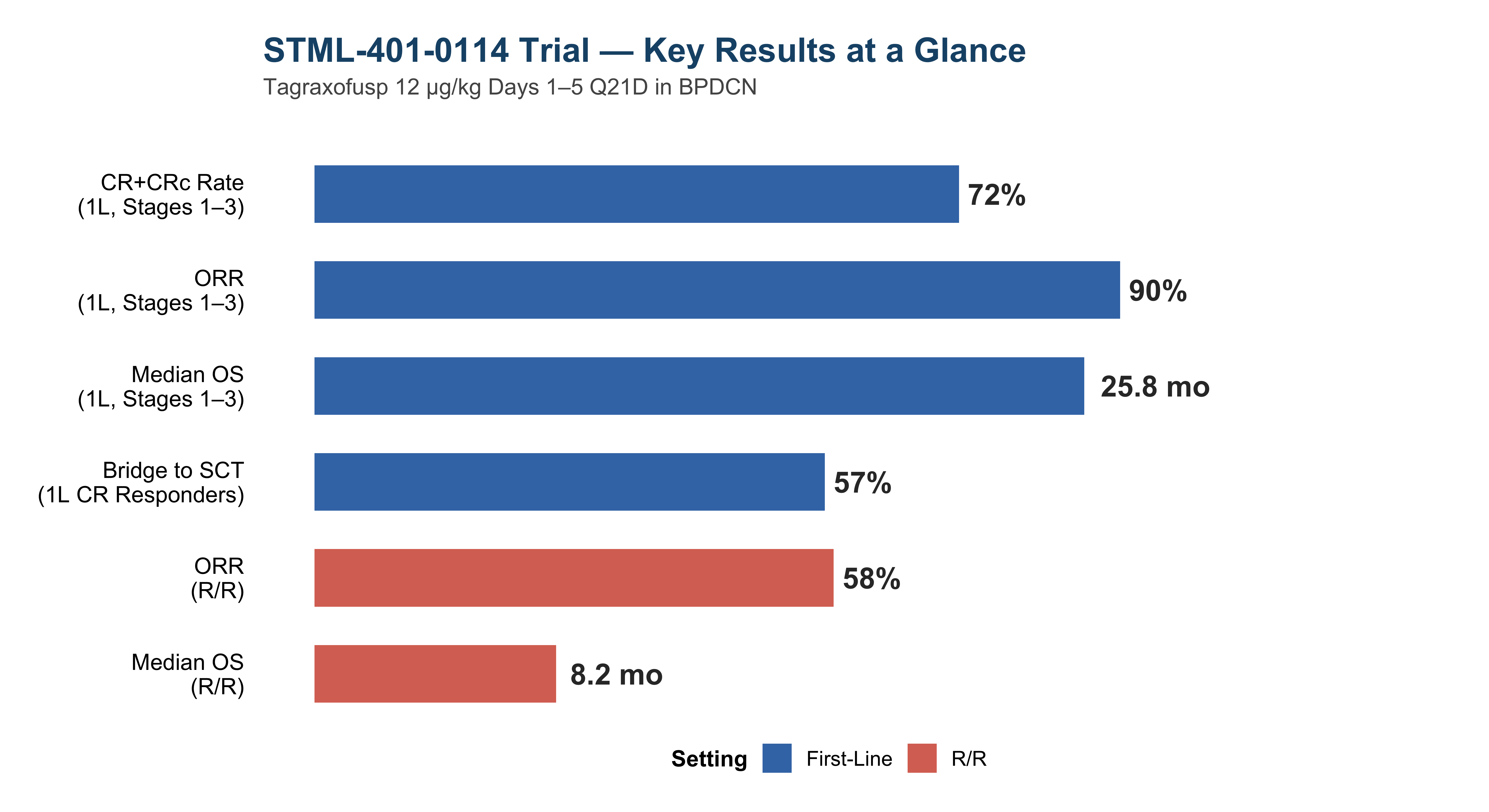
Among 29 previously untreated patients receiving 12 μg/kg (stages 1–3), the CR+CRc rate was 72% (95% CI, 53–87%) and the ORR was 90%, successfully exceeding the null hypothesis threshold of 10%. In the extended cohort of all 65 first-line patients, the CR+CRc rate was 57% with an ORR of 75%.
7.2 Overall Survival — Kaplan-Meier Analysis
Show code
library(ggplot2)
library(dplyr)

km_data <- bind_rows(
  tibble(
    Time = c(0, 3, 6, 9, 12, 15, 18, 21, 24, 27, 30),
    Survival = c(1.00, 0.93, 0.76, 0.69, 0.62, 0.60, 0.59, 0.55, 0.52, 0.48, 0.45),
    Lower    = c(1.00, 0.82, 0.58, 0.50, 0.42, 0.40, 0.38, 0.34, 0.31, 0.28, 0.25),
    Upper    = c(1.00, 0.98, 0.88, 0.83, 0.77, 0.75, 0.74, 0.71, 0.69, 0.65, 0.62),
    Group = "Stages 1–3 (n = 29)\nMedian OS: 25.8 months"
  ),
  tibble(
    Time = c(0, 3, 6, 9, 12, 15, 18, 21, 24, 27, 30),
    Survival = c(1.00, 0.88, 0.70, 0.60, 0.55, 0.52, 0.50, 0.43, 0.40, 0.36, 0.33),
    Lower    = c(1.00, 0.78, 0.56, 0.46, 0.41, 0.38, 0.36, 0.30, 0.27, 0.23, 0.20),
    Upper    = c(1.00, 0.94, 0.80, 0.72, 0.67, 0.64, 0.62, 0.56, 0.53, 0.49, 0.47),
    Group = "All 1L (n = 65)\nMedian OS: 15.8 months"
  ),
  tibble(
    Time = c(0, 3, 6, 9, 12, 15, 18, 21),
    Survival = c(1.00, 0.70, 0.45, 0.33, 0.25, 0.18, 0.12, 0.08),
    Lower    = c(1.00, 0.47, 0.23, 0.14, 0.09, 0.05, 0.02, 0.01),
    Upper    = c(1.00, 0.85, 0.65, 0.53, 0.44, 0.36, 0.28, 0.22),
    Group = "Relapsed/Refractory (n = 19)\nMedian OS: 8.2 months"
  )
)

group_colors_km <- c(
  "Stages 1–3 (n = 29)\nMedian OS: 25.8 months" = "#2166ac",
  "All 1L (n = 65)\nMedian OS: 15.8 months" = "#4393c3",
  "Relapsed/Refractory (n = 19)\nMedian OS: 8.2 months" = "#d6604d"
)

ggplot(km_data, aes(x = Time, y = Survival, color = Group, fill = Group)) +
  geom_ribbon(aes(ymin = Lower, ymax = Upper), alpha = 0.15, color = NA) +
  geom_step(linewidth = 1.3) +
  geom_hline(yintercept = 0.5, linetype = "dashed", color = "grey50", linewidth = 0.5) +
  annotate("text", x = 0.5, y = 0.52, label = "50% survival",
           hjust = 0, size = 3.2, color = "grey40") +
  geom_segment(aes(x = 25.8, xend = 25.8, y = 0, yend = 0.5),
               color = "#2166ac", linetype = "dotted", linewidth = 0.7,
               inherit.aes = FALSE) +
  geom_segment(aes(x = 15.8, xend = 15.8, y = 0, yend = 0.5),
               color = "#4393c3", linetype = "dotted", linewidth = 0.7,
               inherit.aes = FALSE) +
  geom_segment(aes(x = 8.2, xend = 8.2, y = 0, yend = 0.5),
               color = "#d6604d", linetype = "dotted", linewidth = 0.7,
               inherit.aes = FALSE) +
  annotate("text", x = 25.8, y = -0.04, label = "25.8", fontface = "bold",
           color = "#2166ac", size = 3.8) +
  annotate("text", x = 15.8, y = -0.04, label = "15.8", fontface = "bold",
           color = "#4393c3", size = 3.8) +
  annotate("text", x = 8.2, y = -0.04, label = "8.2", fontface = "bold",
           color = "#d6604d", size = 3.8) +
  scale_color_manual(values = group_colors_km) +
  scale_fill_manual(values = group_colors_km) +
  scale_x_continuous(breaks = seq(0, 30, 3), limits = c(0, 32)) +
  scale_y_continuous(
    breaks = seq(0, 1, 0.2),
    labels = scales::percent_format(),
    limits = c(-0.08, 1.05)
  ) +
  labs(
    title = "Overall Survival — Kaplan-Meier Estimates",
    subtitle = "Tagraxofusp 12 μg/kg in BPDCN | Long-term follow-up (median 34 months)",
    x = "Time (months)",
    y = "Overall Survival Probability",
    color = "Population",
    fill = "Population"
  ) +
  theme_minimal(base_size = 14) +
  theme(
    plot.title = element_text(face = "bold", size = 17, color = "#1a5276"),
    plot.subtitle = element_text(size = 12, color = "#555555", margin = margin(b = 15)),
    legend.position = "bottom",
    legend.title = element_text(face = "bold"),
    legend.text = element_text(size = 10),
    panel.grid.minor = element_blank(),
    plot.margin = margin(15, 20, 15, 15)
  )
7.3 Duration of Response and Bridge to SCT
Show code
library(ggplot2)
library(dplyr)
library(tidyr)

# Panel A: Duration of Response
dor_data <- tibble(
  Group = factor(c(
    "Stages 1–3\n(n = 29)",
    "Overall 1L\n(n = 65)",
    "Relapsed/\nRefractory"
  ), levels = c(
    "Stages 1–3\n(n = 29)",
    "Overall 1L\n(n = 65)",
    "Relapsed/\nRefractory"
  )),
  Median_DoR = c(24.9, 24.9, 2.8),
  Lower = c(5.9, 3.8, 0.7),
  Upper = c(30, 30, 14.0),
  NR = c(TRUE, TRUE, FALSE)
)

p_dor <- ggplot(dor_data, aes(x = Group, y = Median_DoR, fill = Group)) +
  geom_col(width = 0.55, alpha = 0.9, show.legend = FALSE) +
  geom_errorbar(aes(ymin = Lower, ymax = ifelse(NR, Median_DoR + 4, Upper)),
                width = 0.15, linewidth = 0.7) +
  geom_text(aes(label = ifelse(NR,
    paste0(Median_DoR, " mo*"), paste0(Median_DoR, " mo"))),
    vjust = -0.8, fontface = "bold", size = 4.5, color = "#333333") +
  annotate("text", x = 2.5, y = 32, label = "*Upper CI: NR",
           fontface = "italic", size = 3, color = "grey50") +
  scale_fill_manual(values = c("#2166ac", "#4393c3", "#d6604d")) +
  scale_y_continuous(limits = c(0, 36), breaks = seq(0, 36, 6)) +
  labs(
    title = "Duration of CR + CRc",
    subtitle = "Median (months)",
    x = NULL, y = "Months"
  ) +
  theme_minimal(base_size = 13) +
  theme(
    plot.title = element_text(face = "bold", size = 14, color = "#1a5276"),
    plot.subtitle = element_text(size = 10, color = "#555555"),
    panel.grid.major.x = element_blank(),
    panel.grid.minor = element_blank(),
    axis.text.x = element_text(size = 10, face = "bold")
  )

# Panel B: Bridge to SCT among responders
sct_data <- tibble(
  Group = factor(c(
    "Stages 1–3\n(n = 29)",
    "Overall 1L\n(n = 65)",
    "Relapsed/\nRefractory"
  ), levels = c(
    "Stages 1–3\n(n = 29)",
    "Overall 1L\n(n = 65)",
    "Relapsed/\nRefractory"
  )),
  SCT_pct = c(57, 51, 5),
  n = c(12, 19, 1),
  N = c(21, 37, 19)
)

p_sct <- ggplot(sct_data, aes(x = Group, y = SCT_pct, fill = Group)) +
  geom_col(width = 0.55, alpha = 0.9, show.legend = FALSE) +
  geom_text(aes(label = paste0(SCT_pct, "%\n(", n, "/", N, ")")),
            vjust = -0.3, fontface = "bold", size = 4, color = "#333333") +
  scale_fill_manual(values = c("#2166ac", "#4393c3", "#d6604d")) +
  scale_y_continuous(limits = c(0, 80), breaks = seq(0, 75, 25),
                     labels = function(x) paste0(x, "%")) +
  labs(
    title = "Bridge to SCT (CR+CRc Responders)",
    subtitle = "Patients proceeding to transplant",
    x = NULL, y = "Patients (%)"
  ) +
  theme_minimal(base_size = 13) +
  theme(
    plot.title = element_text(face = "bold", size = 14, color = "#1a5276"),
    plot.subtitle = element_text(size = 10, color = "#555555"),
    panel.grid.major.x = element_blank(),
    panel.grid.minor = element_blank(),
    axis.text.x = element_text(size = 10, face = "bold")
  )

library(gridExtra)
grid.arrange(p_dor, p_sct, ncol = 2)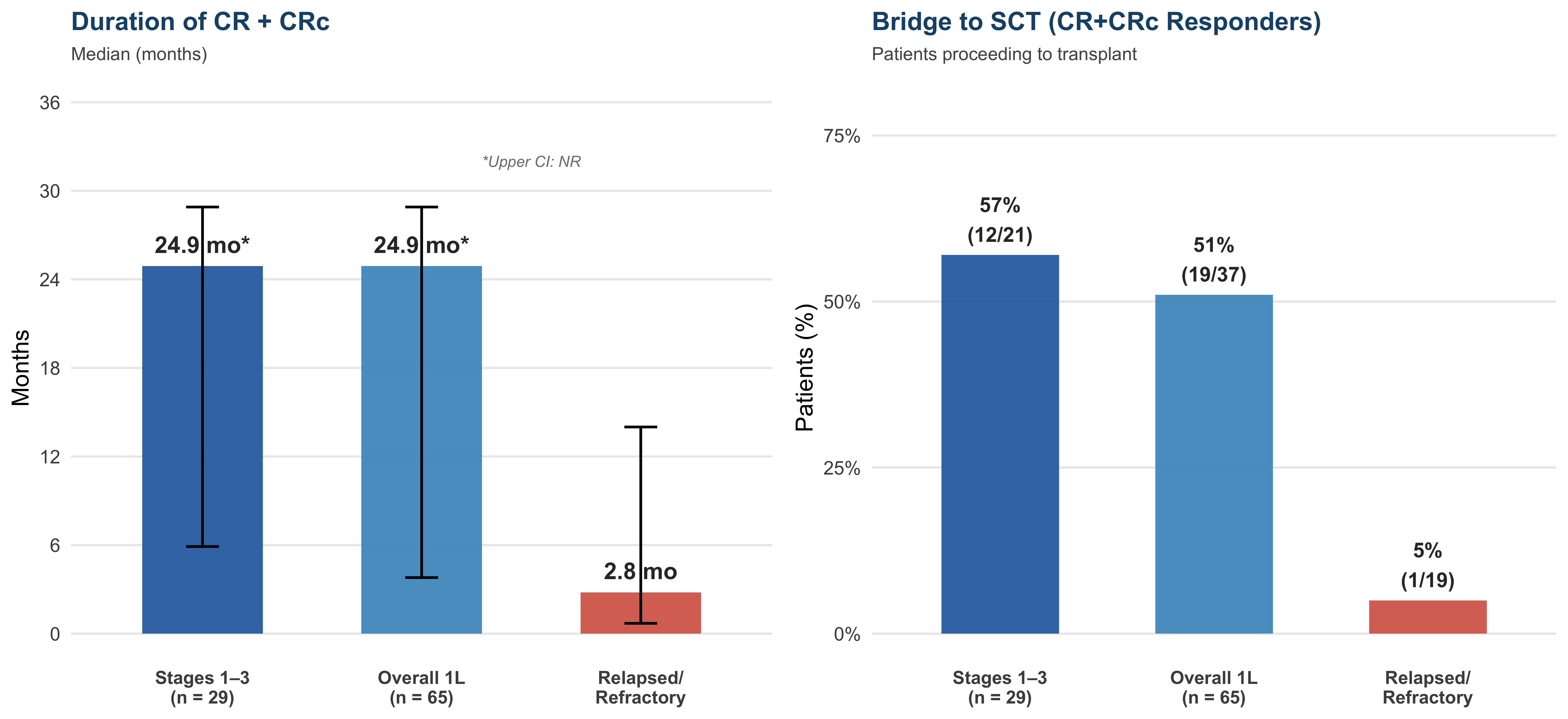
7.4 Landmark Survival Rates
Show code
import matplotlib.pyplot as plt
import numpy as np

groups = ['Stages 1–3\n(n = 29)', 'Overall 1L\n(n = 65)', 'Relapsed/Refractory\n(n = 19)']
os_12mo = [62, 55, 25]
os_18mo = [59, 50, 18]
os_24mo = [52, 40, 8]

x = np.arange(len(groups))
width = 0.22

fig, ax = plt.subplots(figsize=(11, 5.5))

bars1 = ax.bar(x - width, os_12mo, width, label='12-Month OS',
               color='#2166ac', alpha=0.9, edgecolor='white', linewidth=1)
bars2 = ax.bar(x, os_18mo, width, label='18-Month OS',
               color='#4393c3', alpha=0.9, edgecolor='white', linewidth=1)
bars3 = ax.bar(x + width, os_24mo, width, label='24-Month OS',
               color='#67a9cf', alpha=0.9, edgecolor='white', linewidth=1)

for bar, val in zip(bars1, os_12mo):
    ax.text(bar.get_x() + bar.get_width()/2, bar.get_height() + 2,
            f'{val}%', ha='center', va='bottom', fontweight='bold', fontsize=10,
            color='#2166ac')

for bar, val in zip(bars2, os_18mo):
    ax.text(bar.get_x() + bar.get_width()/2, bar.get_height() + 2,
            f'{val}%', ha='center', va='bottom', fontweight='bold', fontsize=10,
            color='#4393c3')

for bar, val in zip(bars3, os_24mo):
    ax.text(bar.get_x() + bar.get_width()/2, bar.get_height() + 2,
            f'{val}%', ha='center', va='bottom', fontweight='bold', fontsize=10,
            color='#67a9cf')

ax.set_xticks(x)
ax.set_xticklabels(groups, fontsize=11, fontweight='bold')
ax.set_ylabel('Overall Survival (%)', fontsize=12)
ax.set_ylim(0, 80)
(0.0, 80.0)Show code
ax.set_title('Landmark Overall Survival Rates',
             fontsize=16, fontweight='bold', color='#1a5276', pad=15)
ax.legend(fontsize=11, frameon=False, loc='upper right')
ax.spines['top'].set_visible(False)
ax.spines['right'].set_visible(False)
ax.grid(axis='y', alpha=0.3, linestyle='--')

plt.tight_layout()
plt.show()
8 Safety Profile
8.1 Adverse Events Overview
Show code
import matplotlib.pyplot as plt
import numpy as np
import seaborn as sns

aes = [
    'ALT increased', 'AST increased', 'Hypoalbuminemia',
    'Peripheral edema', 'Thrombocytopenia', 'Fatigue',
    'Nausea', 'Pyrexia', 'Weight increased',
    'Hyperglycemia', 'Chills', 'Hypotension',
    'Headache', 'Back pain', 'Appetite decreased',
    'Anemia', 'Constipation', 'Capillary leak syndrome',
    'Hyponatremia'
]

treatment_naive = [69, 66, 44, 41, 50, 41, 47, 34, 41, 34, 28, 22, 34, 22, 22, 25, 31, 16, 16]
previously_treated = [53, 47, 80, 73, 47, 53, 40, 67, 33, 40, 47, 40, 7, 33, 33, 20, 7, 27, 27]
all_patients = [64, 60, 55, 51, 49, 45, 45, 45, 38, 36, 34, 28, 26, 26, 26, 23, 23, 19, 19]

data = np.array([treatment_naive, previously_treated, all_patients]).T

fig, ax = plt.subplots(figsize=(10, 10))

cmap = sns.color_palette("YlOrRd", as_cmap=True)

im = ax.imshow(data, cmap=cmap, aspect='auto', vmin=0, vmax=80)

for i in range(len(aes)):
    for j in range(3):
        val = data[i, j]
        color = 'white' if val > 50 else '#333333'
        ax.text(j, i, f'{val}%', ha='center', va='center',
                fontsize=10, fontweight='bold', color=color)

ax.set_xticks([0, 1, 2])
ax.set_xticklabels(
    ['Treatment-Naïve\n(n = 32)', 'Previously Treated\n(n = 15)',
     'All Patients\n(N = 47)'],
    fontsize=11, fontweight='bold'
)
ax.set_yticks(range(len(aes)))
ax.set_yticklabels(aes, fontsize=11)
ax.xaxis.set_ticks_position('top')
ax.xaxis.set_label_position('top')

cbar = plt.colorbar(im, ax=ax, shrink=0.6, label='Patients (%)')

ax.set_title('Treatment-Emergent Adverse Events (≥15% Any Grade)',
             fontsize=15, fontweight='bold', color='#1a5276', pad=60)

plt.tight_layout()
plt.show()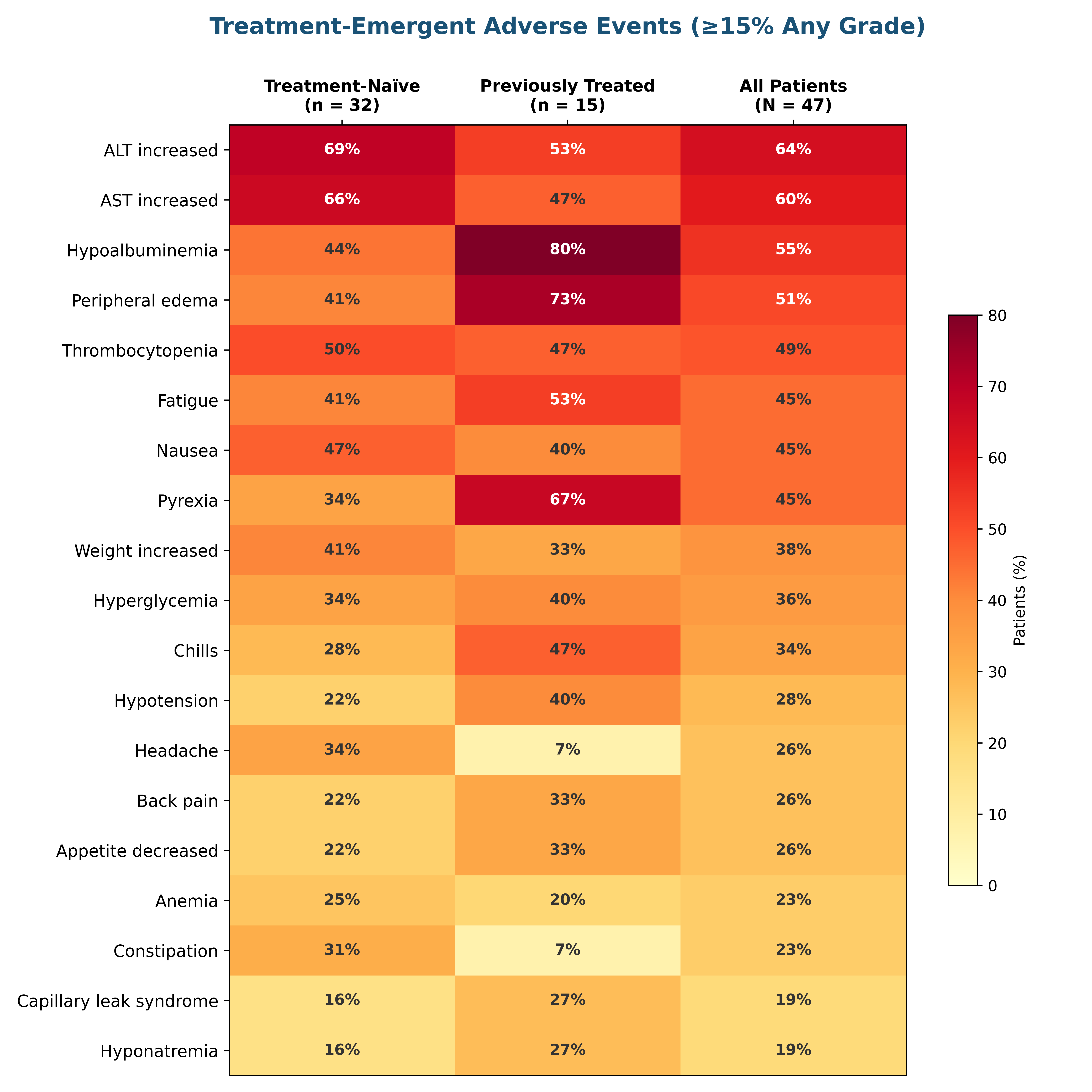
8.2 Grade ≥3 Adverse Events
Show code
library(ggplot2)
library(dplyr)

grade3_data <- tibble(
  AE = c(
    "Thrombocytopenia",
    "ALT increased",
    "AST increased",
    "Capillary leak syndrome\n(Grade ≥3)"
  ),
  Percentage = c(33, 32, 30, 7)
) |>
  mutate(AE = factor(AE, levels = rev(AE)))

ggplot(grade3_data, aes(x = Percentage, y = AE)) +
  geom_segment(aes(x = 0, xend = Percentage, yend = AE),
               color = "#d6604d", linewidth = 1.5) +
  geom_point(size = 6, color = "#d6604d") +
  geom_text(aes(label = paste0(Percentage, "%")),
            hjust = -0.6, fontface = "bold", size = 4, color = "#333333") +
  scale_x_continuous(limits = c(0, 45), breaks = seq(0, 40, 10),
                     labels = function(x) paste0(x, "%")) +
  labs(
    title = "Grade ≥3 Adverse Events",
    subtitle = "Long-term safety population (N = 89)",
    x = "Patients (%)",
    y = NULL
  ) +
  theme_minimal(base_size = 13) +
  theme(
    plot.title = element_text(face = "bold", size = 16, color = "#1a5276"),
    plot.subtitle = element_text(size = 11, color = "#555555", margin = margin(b = 15)),
    panel.grid.major.y = element_blank(),
    panel.grid.minor = element_blank(),
    axis.text.y = element_text(size = 11),
    plot.margin = margin(15, 30, 15, 15)
  )
8.3 Special Safety Topics
Show code
library(knitr)

safety_special <- data.frame(
  Event = c(
    "Capillary Leak Syndrome",
    "Capillary Leak Syndrome",
    "Capillary Leak Syndrome",
    "Capillary Leak Syndrome",
    "Capillary Leak Syndrome",
    "Capillary Leak Syndrome",
    "Hepatotoxicity",
    "Hepatotoxicity",
    "Thrombocytopenia",
    "Temporal Pattern"
  ),
  Detail = c(
    "Overall incidence: 21% (long-term follow-up, N = 89)",
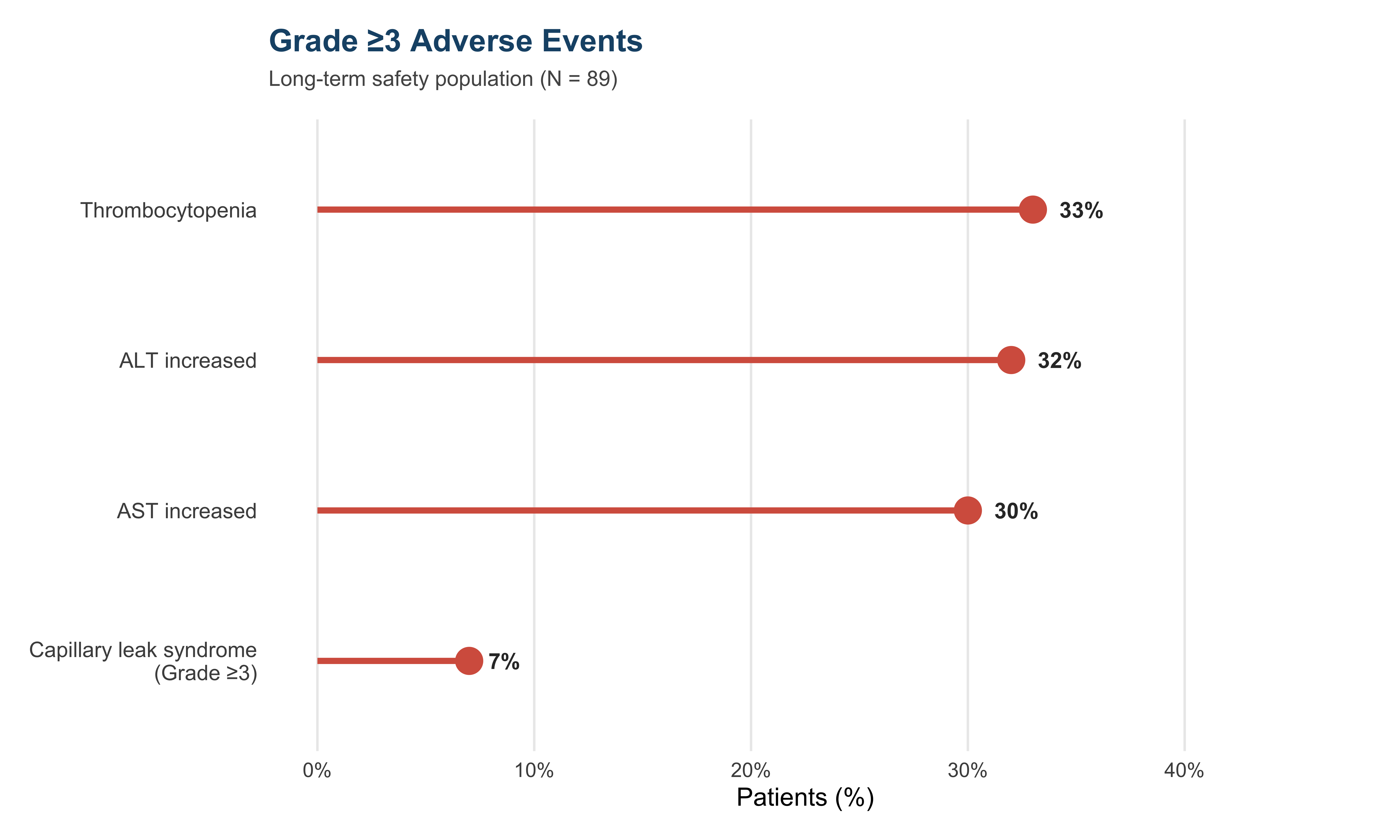
    "Grade ≥3: 7% (including 3 fatal events across all stages)",
    "Median time to onset: 6 days (range 3–51)",
    "Median duration: 6 days (range 3–69)",
    "Almost exclusively Cycle 1; does not recur",
    "Management: IV albumin (goal ≥3.5 g/dL), IV steroids, fluid management",
    "ALT/AST elevations in >60% of patients; Grade ≥3 in ~30%",
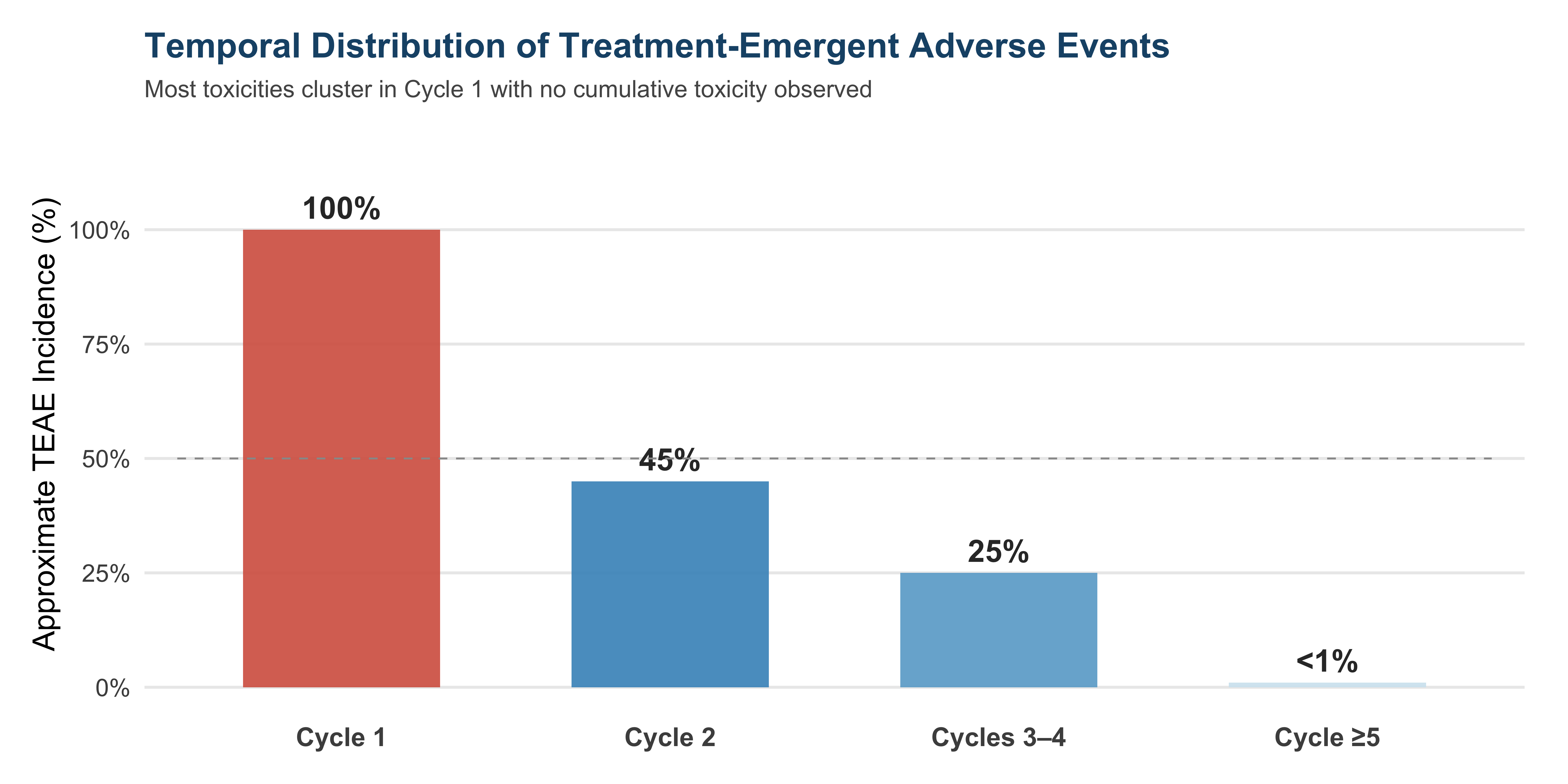
    "Transient, restricted to Cycle 1; no cumulative hepatotoxicity",
    "Any grade: 43%; Grade ≥3: 33% — most common severe AE",
    "<1% of patients experienced any TEAE in Cycle ≥5"
  )
)

kable(safety_special,
      col.names = c("Event", "Key Details"),
align = c("l", "l"))| Event | Key Details |
|---|---|
| Capillary Leak Syndrome | Overall incidence: 21% (long-term follow-up, N = 89) |
| Capillary Leak Syndrome | Grade ≥3: 7% (including 3 fatal events across all stages) |
| Capillary Leak Syndrome | Median time to onset: 6 days (range 3–51) |
| Capillary Leak Syndrome | Median duration: 6 days (range 3–69) |
| Capillary Leak Syndrome | Almost exclusively Cycle 1; does not recur |
| Capillary Leak Syndrome | Management: IV albumin (goal ≥3.5 g/dL), IV steroids, fluid management |
| Hepatotoxicity | ALT/AST elevations in >60% of patients; Grade ≥3 in ~30% |
| Hepatotoxicity | Transient, restricted to Cycle 1; no cumulative hepatotoxicity |
| Thrombocytopenia | Any grade: 43%; Grade ≥3: 33% — most common severe AE |
| Temporal Pattern | <1% of patients experienced any TEAE in Cycle ≥5 |
8.4 Toxicity Temporal Profile
Show code
library(ggplot2)

timing_data <- data.frame(
  cycle = factor(c("Cycle 1", "Cycle 2", "Cycles 3–4", "Cycle ≥5"),
                 levels = c("Cycle 1", "Cycle 2", "Cycles 3–4", "Cycle ≥5")),
  incidence = c(100, 45, 25, 1)
)

ggplot(timing_data, aes(x = cycle, y = incidence)) +
  geom_col(fill = c("#d6604d", "#4393c3", "#67a9cf", "#d1e5f0"),
           width = 0.6, alpha = 0.9) +
  geom_text(aes(label = paste0(ifelse(incidence == 1, "<1", incidence), "%")),
            vjust = -0.5, fontface = "bold", size = 5, color = "#333333") +
  annotate("segment", x = 0.5, xend = 4.5, y = 50, yend = 50,
           linetype = "dashed", color = "grey60", linewidth = 0.4) +
  scale_y_continuous(limits = c(0, 115), breaks = seq(0, 100, 25),
                     labels = function(x) paste0(x, "%")) +
  labs(
    title = "Temporal Distribution of Treatment-Emergent Adverse Events",
    subtitle = "Most toxicities cluster in Cycle 1 with no cumulative toxicity observed",
    x = NULL,
    y = "Approximate TEAE Incidence (%)"
  ) +
  theme_minimal(base_size = 14) +
  theme(
    plot.title = element_text(face = "bold", size = 16, color = "#1a5276"),
    plot.subtitle = element_text(size = 11, color = "#555555", margin = margin(b = 15)),
    panel.grid.major.x = element_blank(),
    panel.grid.minor = element_blank(),
    axis.text.x = element_text(size = 12, face = "bold"),
    plot.margin = margin(15, 20, 15, 15)
  )
9 Comparative Context
Show code
import matplotlib.pyplot as plt
import numpy as np

fig, axes = plt.subplots(1, 3, figsize=(14, 5.5))

# Panel A: Response rates
drugs = ['Tagraxofusp\n(Pivotal)', 'PVEK\n(CADENZA)']
ccr = [72, 75]
orr = [90, 80]

x = np.arange(len(drugs))
w = 0.3
axes[0].bar(x - w/2, ccr, w, label='CR+CRc', color='#2166ac', alpha=0.9)
axes[0].bar(x + w/2, orr, w, label='ORR', color='#67a9cf', alpha=0.9)

for i, (c, o) in enumerate(zip(ccr, orr)):
    axes[0].text(i - w/2, c + 2, f'{c}%', ha='center', fontweight='bold', fontsize=11, color='#2166ac')
    axes[0].text(i + w/2, o + 2, f'{o}%', ha='center', fontweight='bold', fontsize=11, color='#67a9cf')

axes[0].set_xticks(x)
axes[0].set_xticklabels(drugs, fontsize=11, fontweight='bold')
axes[0].set_ylabel('Response Rate (%)', fontsize=11)
axes[0].set_ylim(0, 110)
(0.0, 110.0)Show code
axes[0].set_title('Frontline Response Rates', fontsize=13, fontweight='bold', color='#1a5276')
axes[0].legend(fontsize=9, frameon=False)
axes[0].spines['top'].set_visible(False)
axes[0].spines['right'].set_visible(False)

# Panel B: Dosing comparison
labels = ['Tagraxofusp', 'PVEK']
infusion_days = [5, 1]
colors_dose = ['#2166ac', '#d6604d']
axes[1].bar(labels, infusion_days, color=colors_dose, width=0.5, alpha=0.9)
for i, v in enumerate(infusion_days):
    axes[1].text(i, v + 0.15, f'{v} day{"s" if v > 1 else ""}',
                ha='center', fontweight='bold', fontsize=12)
axes[1].set_ylabel('Infusion Days per Cycle', fontsize=11)
axes[1].set_ylim(0, 7)
(0.0, 7.0)Show code
axes[1].set_title('Dosing Schedule', fontsize=13, fontweight='bold', color='#1a5276')
axes[1].spines['top'].set_visible(False)
axes[1].spines['right'].set_visible(False)

# Panel C: Key AEs
ae_labels = ['CLS', 'Peripheral\nEdema', 'ALT/AST\nElevation']
tagra_ae = [21, 51, 64]
pvek_ae = [0, 54, 5]

x_ae = np.arange(len(ae_labels))
axes[2].bar(x_ae - w/2, tagra_ae, w, label='Tagraxofusp', color='#2166ac', alpha=0.9)
axes[2].bar(x_ae + w/2, pvek_ae, w, label='PVEK', color='#d6604d', alpha=0.9)
for i, (t, p) in enumerate(zip(tagra_ae, pvek_ae)):
    if t > 0:
        axes[2].text(i - w/2, t + 1.5, f'{t}%', ha='center', fontsize=10,
                    fontweight='bold', color='#2166ac')
    if p > 0:
        axes[2].text(i + w/2, p + 1.5, f'{p}%', ha='center', fontsize=10,
                    fontweight='bold', color='#d6604d')

axes[2].set_xticks(x_ae)
axes[2].set_xticklabels(ae_labels, fontsize=10, fontweight='bold')
axes[2].set_ylabel('Incidence (%)', fontsize=11)
axes[2].set_ylim(0, 80)
(0.0, 80.0)Show code
axes[2].set_title('Key Safety Signals', fontsize=13, fontweight='bold', color='#1a5276')
axes[2].legend(fontsize=9, frameon=False)
axes[2].spines['top'].set_visible(False)
axes[2].spines['right'].set_visible(False)

fig.text(0.5, -0.02,
         '⚠ Cross-trial comparisons should be interpreted with caution due to differences in study design and patient populations.',
         ha='center', fontsize=9, fontstyle='italic', color='#888888')

plt.suptitle('Tagraxofusp vs. PVEK — Contextual Comparison (Frontline BPDCN)',
             fontsize=16, fontweight='bold', color='#1a5276', y=1.03)
plt.tight_layout()
plt.show()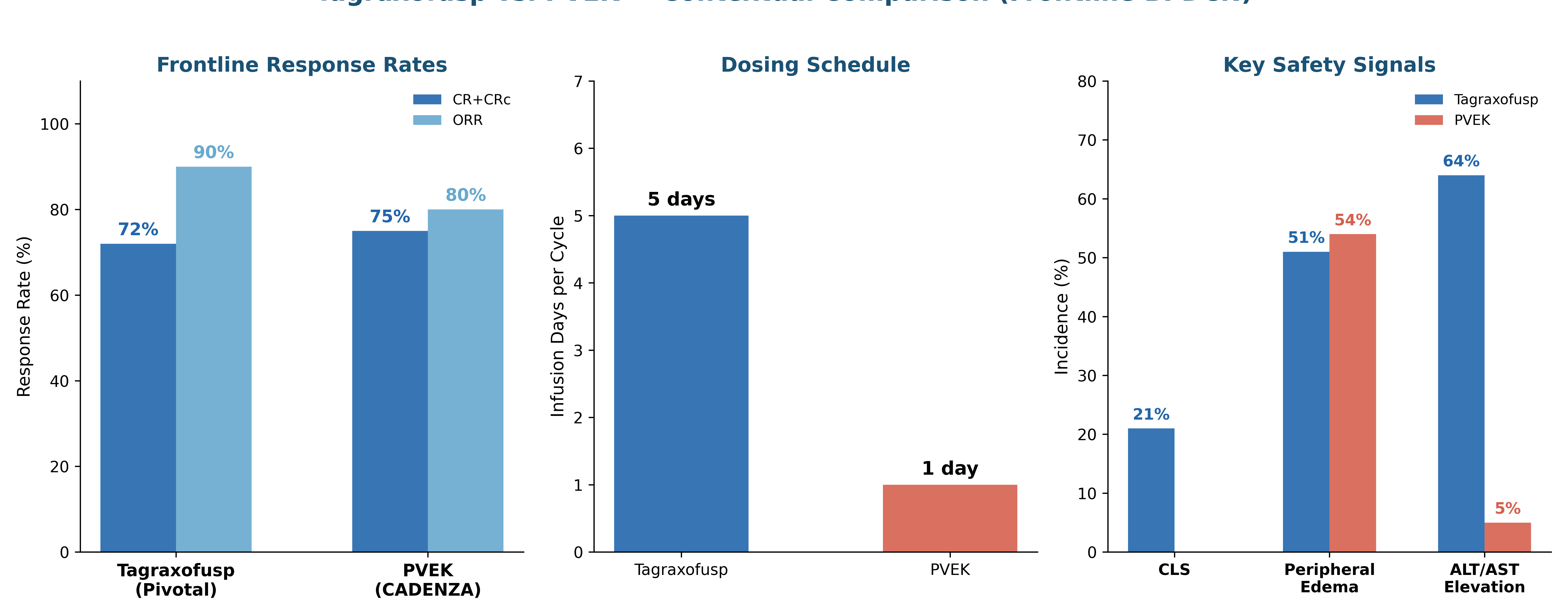
10 Summary & Implications
Show code
library(ggplot2)

summary_data <- data.frame(
  Metric = factor(c(
    "CR+CRc Rate\n(1L, Stages 1–3)",
    "ORR\n(1L, Stages 1–3)",
    "Median OS\n(1L, Stages 1–3)",
    "Bridge to SCT\n(1L CR Responders)",
    "ORR\n(R/R)",
    "Median OS\n(R/R)"
  ), levels = rev(c(
    "CR+CRc Rate\n(1L, Stages 1–3)",
    "ORR\n(1L, Stages 1–3)",
    "Median OS\n(1L, Stages 1–3)",
    "Bridge to SCT\n(1L CR Responders)",
    "ORR\n(R/R)",
    "Median OS\n(R/R)"
  ))),
  Value = c(72, 90, 25.8, 57, 58, 8.2),
  Unit = c("%", "%", "months", "%", "%", "months"),
  Category = c("First-Line", "First-Line", "First-Line", "First-Line", "R/R", "R/R"),
  Display = c("72%", "90%", "25.8 mo", "57%", "58%", "8.2 mo"),
  bar_val = c(72, 90, 86, 57, 58, 27)
)

ggplot(summary_data, aes(x = bar_val, y = Metric, fill = Category)) +
  geom_col(width = 0.6, alpha = 0.9) +
  geom_text(aes(label = Display), hjust = -0.15,
            fontface = "bold", size = 5.5, color = "#333333") +
  scale_fill_manual(
    values = c("First-Line" = "#2166ac", "R/R" = "#d6604d"),
    name = "Setting"
  ) +
  scale_x_continuous(limits = c(0, 115)) +
  labs(
    title = "STML-401-0114 Trial — Key Results at a Glance",
    subtitle = "Tagraxofusp 12 μg/kg Days 1–5 Q21D in BPDCN",
    x = NULL, y = NULL
  ) +
  theme_void(base_size = 14) +
  theme(
    plot.title = element_text(face = "bold", size = 18, color = "#1a5276",
                              margin = margin(b = 5)),
    plot.subtitle = element_text(size = 12, color = "#555555",
                                 margin = margin(b = 20)),
    axis.text.y = element_text(size = 12, hjust = 1, margin = margin(r = 10)),
    legend.position = "bottom",
    legend.title = element_text(face = "bold", size = 12),
    legend.text = element_text(size = 11),
    plot.margin = margin(20, 50, 20, 20)
  )
Sources: Pemmaraju N, Lane AA, Sweet KL, et al. Tagraxofusp in Blastic Plasmacytoid Dendritic-Cell Neoplasm. N Engl J Med. 2019;380(17):1628-37. DOI: 10.1056/NEJMoa1815105. Pemmaraju N, Sweet KL, Stein AS, et al. Long-Term Benefits of Tagraxofusp for Patients With BPDCN. J Clin Oncol. 2022;40(26):3032-36. Luskin MR, Lane AA. Tagraxofusp for BPDCN. Haematologica. 2024;109(1):44-52. ClinicalTrials.gov: NCT02113982.